Introduction to Statistical Learning

Let \(X\) be the vector of all your features (i.e. \(X=(X_{1}, X_{2},\dots, X_{p})\), then the output is:

\begin{equation*} Y=f(X)+\epsilon \end{equation*}

\(\epsilon\) is called the error term, and it is random - the mean is 0. \(f\) represents the systematic information.

The above equation is the “true” equation. The problem is that \(f\) is unknown. So we estimate it by \(\hat{f}\):

\begin{equation*} \hat{Y}=\hat{f}(X) \end{equation*}

We use two terms to specify the error in our model. There is the reducible error which is the error in estimating \(f\). In principle, we can bring this error down to 0. The other error is \(\epsilon\) and is called the irreducible error. This is because even if we guess the true \(f\), there is still variation in reality, so we’ll never get the exact answer.

In the analysis above, when I write \(f\) as being the “real” relationship, what I mean is the real relationship with the \(p\) features. The output may depend on more features than what we have, and the error due to this is lumped into \(\epsilon\).

Now:

\begin{equation*} E\left[\left(Y-\hat{Y}\right)^{2}\right]=E\left[\left(f(X)+\epsilon-\hat{f}(X)\right)^{2}\right] \end{equation*}

\begin{equation*} E\left[\left(Y-\hat{Y}\right)^{2}\right]=E\left[\left(f(X)-\hat{f}(X)\right)^{2}\right] + \sigma_{\epsilon}^{2} \end{equation*}

The first term refers to the reducible error, and the second term refers to the irreducible error.

You can derive this using the identity: \(\sigma_{Y}^{2}=E[Y^{2}]-(E[Y])^{2}\)

Common questions we ask:

Which predictors are associated with the response?
What is the relationship between the response and each predictor?

Most statistical learning tasks involve either parametric or non-parametric approaches.

Parametric approaches assume a functional form for \(f\), and then we proceed to estimate the parameters. In a non-parametric approach, we don’t assume a form for \(f\). That doesn’t mean we don’t give it a form - it just means we don’t believe that it is anything resembling reality. The upshot is that non-parametric approaches are a lot more flexible, but more prone to overfitting. They may be less interpretable, and they often need a lot more training points. An example is using splines.

Assessing Model Accuracy

For a regression problem, the most common way to assess the accuracy of a model is the mean square error:

\begin{equation*} MSE=\frac{1}{n}\sum_{i=1}^{n}\left(y_{i}-\hat{f}(x_{i})^{2}\right) \end{equation*}

Of course, we calculate the Mean Square Error on both the test and training sets, and plot both vs the flexibility of our models. We’ll usually get a curve like this:

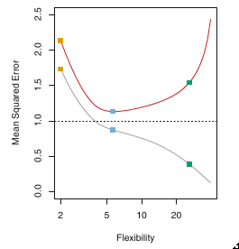
Test vs Training Error Curve vs Flexibility

The red curve is the test error curve. When it starts going up, you know you are overfitting. In fact, the book defines overfitting as the case where a less flexible model would have yielded a smaller test Mean Square Error.

Whatever machine learning problem you work on, make sure you plot this curve!

Bias-Variance Tradeoff

Suppose we have a value \(x_{0}\) in the test set. We pick a model, and train it over several randomly chosen training sets. We want to calculate the mean square error averaged over all the training sets for that one point. In other words, we want to calculate:

\begin{equation*} E\left[\left(y_{0}-\hat{f}(x_{0})\right)^{2}\right] \end{equation*}

where we are fixing \(x_{0}\) and averaging over all training sets.

Now: \(y_{0}=f(x_{0})+\epsilon\). We know that \(f(x_{0})\) is a constant, so the only thing that varies is \(\epsilon\). So \(\sigma_{y_{0}}^{2}=\sigma_{\epsilon}^{2}\) and the mean of \(y_{0}\) is \(f(x_{0})\).

\begin{equation*} E\left[\left(y_{0}-\hat{f}(x_{0})\right)^{2}\right]=V\left[y_{0}-\hat{f}(x_{0})\right]+\left[E\left[y_{0}-\hat{f}(x_{0})\right]\right]^{2} \end{equation*}

\begin{equation*} E\left[\left(y_{0}-\hat{f}(x_{0})\right)^{2}\right]=V[\epsilon]+V\left[\hat{f}(x_{0})\right]+\left[f(x_{0})-E\left[\hat{f}(x_{0})\right]\right]^{2} \end{equation*}

The last term is referred to as the bias. Qualitatively, it represents the error in picking the wrong model for \(f\). It is a measure of how off we are regardless of our training set.

The second term is a measure of how much our prediction varies with the choice of training set. How sensitive is it to our training data?

So to minimize the error, we need to find a model that minimizes the variance in our prediction as well as the bias. The relative change of variance and bias will specify whether our test mean square error goes up or down.

Generally, more flexible models have a lower bias and a higher variance.

In general, this is referred to as the bias-variance tradeoff.

Classification

Instead of the mean square error, we use the error rate:

\begin{equation*} \frac{1}{n}\sum_{i=1}^{n}I\left(y_{i}\ne \hat{y}_{i}\right) \end{equation*}

In words, this is the fraction of the predictions that were wrong. \(I\) is just the indicator function.

The test error rate shown above is minimized (on average), by a classifier that assigns each observation to its most likely class. So:

\begin{equation*} P(Y=j|X=x_{0}) \end{equation*}

Pick the \(j\) that maximizes this quantity. This is the Bayes classifier.

For the test set, we use a different metric. For a given point, the metric is:

\begin{equation*} 1-\max_{j}P(Y=j|X=x_{0}) \end{equation*}

Note that even if our classifier predicts \(j\) correctly, this may be non-zero. For the full test set, it is:

\begin{equation*} 1-E\left(\max_{j}P(Y=j|X)\right) \end{equation*}

I imagine the reason we use this and not the fraction is that this could be a continuous variable.

The problem with this approach is that we don’t know the distribution, so calculating the probability is impossible.

KNN Classifier

The KNN Classifier is one where we estimate the probability distribution. The concept is simple: Pick \(K\). Then for any given \(x_{0}\), find the \(K\) nearest points in the training set. Then the probability of \(x_{0}\) being in class \(j\) is just the fraction of points in the \(K\) neighborhood that are in class \(j\).

In practice, KNN can often get quite close to the Bayes classifier. But your choice of \(K\) can really impact the variance.